SonoSK

An open-source Python library for medical ultrasound. Design a probe, place it in front of a tissue phantom, and get the B-mode image, or heat a target and see the temperature, the thermal dose and the lesion left behind.

pip install sonosk

Get started Read the documentation See the examples

Simulated B-mode image with an anechoic cyst, two lesions and a row of wire targets — Simulated image of a test phantom: 128-element linear array at 5 MHz, nine plane waves compounded.

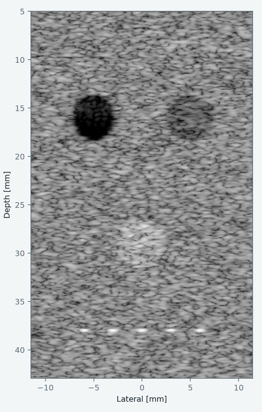
What it simulates

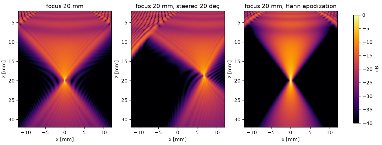
Transducers: Flat and focused elements, annular arrays, linear and phased arrays with an elevation lens, convex and endocavity arrays, matrix arrays and line-focus sources, with focusing, steering and apodization.
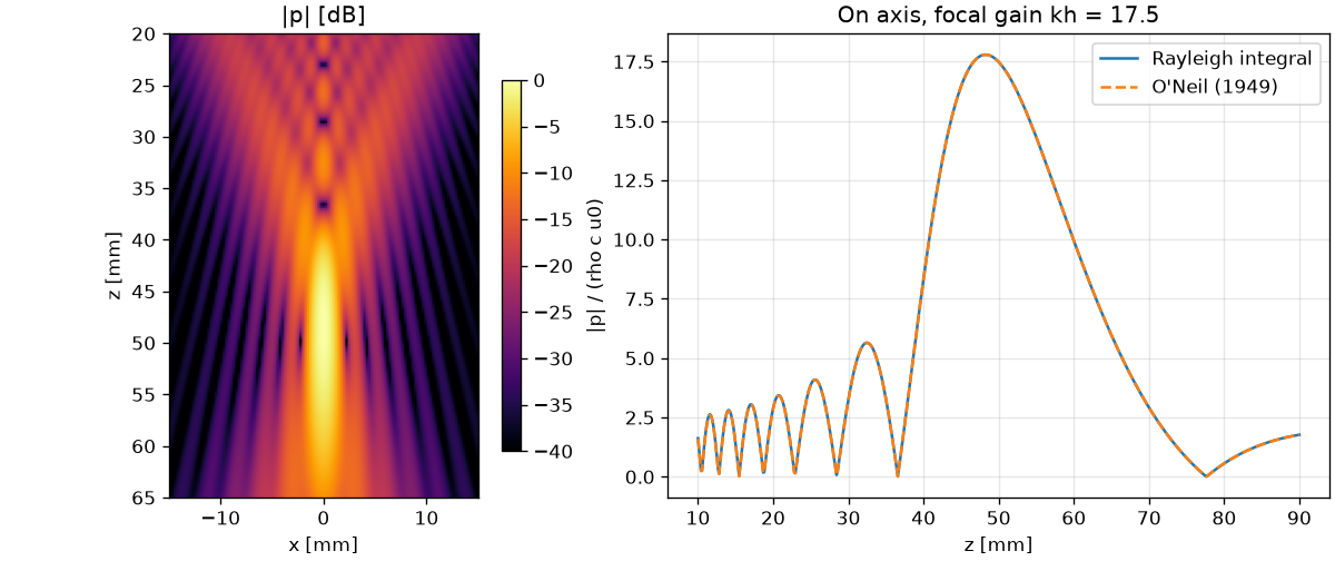
Pressure fields: Rayleigh integral in an attenuating medium and the angular spectrum method, on lines, planes and volumes.
Imaging: Pulse-echo signals from scatterer phantoms, plane, diverging and focused transmits, delay-and-sum beamforming and compounding.
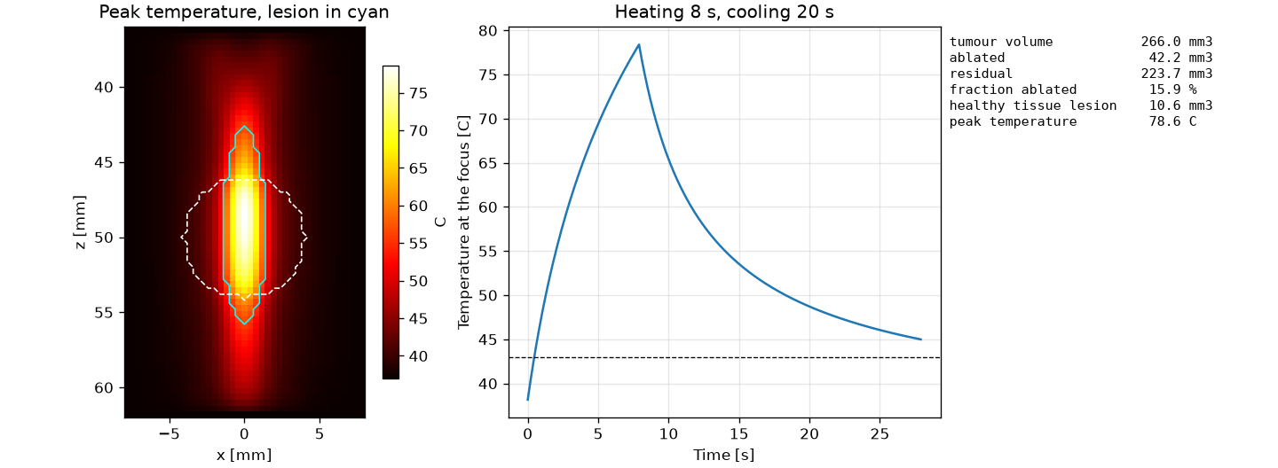
Therapy: Heat from the field, the Pennes bioheat equation in 1, 2 and 3 dimensions, CEM43 dose, lesion maps, and the ablated and residual target.
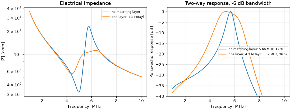
Probe design: Mason model of a piezoelectric element with backing and matching layers: impedance, transmit and pulse-echo response.
Safety and quality: Mechanical index, derated intensities and FDA limits; resolution, contrast, CNR, gCNR and speckle statistics.

Figures made with SonoSK

Peak temperature around a focused ultrasound exposure with lesion and tumour outlines — Ablation of a 4 mm tumour by a 1 MHz focused bowl: peak temperature, lesion outline and the part of the tumour left untreated.

Focused, steered and apodized beams of a linear array — Beams of a linear array: focused, steered by 20 degrees, and with a Hann apodization.

Field of a focused bowl and its on-axis amplitude against the O'Neil solution — Field of a focused bowl, checked against O'Neil's closed-form solution on the axis.

Impedance and pulse-echo response of a piezoelectric element with and without a matching layer — A 5.7 MHz element with and without a quarter-wave matching layer: the two-way bandwidth grows from 12 % to 36 %.

A first simulation

import sonosk as sk
from sonosk import field, transducer

probe = transducer.linear_array(128, pitch=0.3e-3, height=5e-3, elev_focus=20e-3)
probe.focus((0, 0, 20e-3), c=1540.0)

grid = sk.Grid.centered((121, 151), 0.2e-3, depth_start=2e-3)
p = field.rayleigh_grid(probe, grid, f=5e6, c=1540.0, alpha0=0.5)

The getting started page continues from here to a phantom, an image, its quality measures and a heating exposure. Each solver is checked against a closed-form result; the comparisons are on the validation page, and the plan for tissue data and organ phantoms is on the roadmap.

Citing SonoSK

Kooklan S. SonoSK: medical ultrasound simulation in Python. Zenodo, 2026. doi:10.5281/zenodo.23517377

This DOI always resolves to the latest release, and every release has its own DOI as well. BibTeX and the DOI of each version are on the citing page.