Examples

Each figure in this guide comes from a script in the examples folder of the repository. Run a script to see the figure and the printed numbers:

pip install "sonosk[plot]"
python examples/bmode_phantom.py

Material values in the examples are generic numbers chosen to show the method. They are not measured tissue data.

B-mode image of a test phantom

Background speckle, an anechoic cyst, a -10 dB and a +6 dB lesion and a row of wire targets, imaged by a 128-element linear array at 5 MHz with nine compounded plane waves.

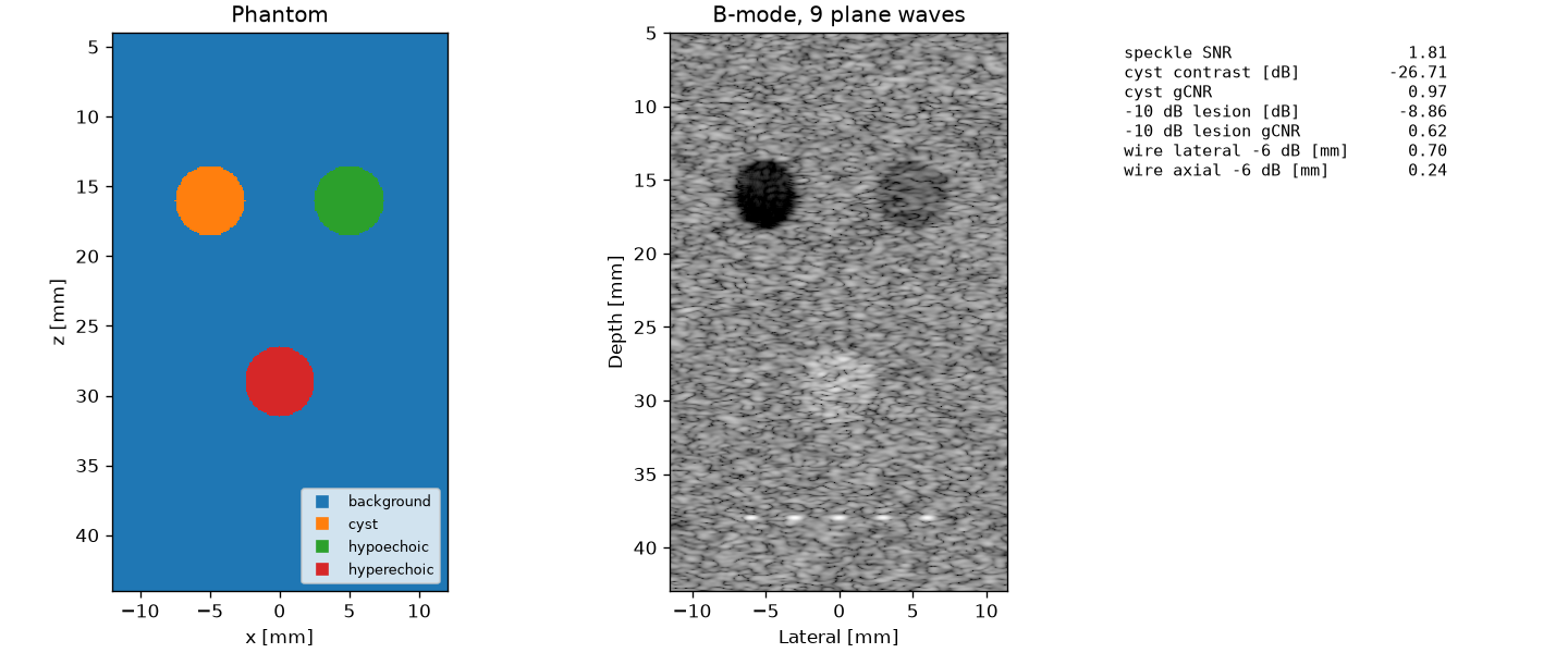
"""B-mode image of a test phantom with plane-wave compounding.

The phantom has a background of fully developed speckle, an anechoic cyst,
a -10 dB lesion, a +6 dB lesion and a row of wire targets. A 128-element
linear array at 5 MHz sends 9 plane waves between -12 and +12 degrees.
The table lists the quality measures of the image.

The material values are generic soft-tissue numbers for the example.
"""

import matplotlib.pyplot as plt
import numpy as np

import sonosk as sk
import sonosk.plot as splt
from sonosk import imaging, phantom, quality, transducer

F0 = 5e6
C = 1540.0
CYST = (-5e-3, 0, 16e-3)
DARK = (5e-3, 0, 16e-3)
BRIGHT = (0.0, 0, 29e-3)
R = 2.5e-3


def compute(seed=0):
    g = sk.Grid.centered((241, 401), 0.1e-3, depth_start=4e-3)
    mats = [sk.Material("background", C, 1000, alpha0=0.5, echo=0.0),
            sk.Material("cyst", C, 1000, alpha0=0.5, echo=-np.inf),
            sk.Material("hypoechoic", C, 1000, alpha0=0.5, echo=-10.0),
            sk.Material("hyperechoic", C, 1000, alpha0=0.5, echo=6.0)]
    lab = np.zeros(g.shape, int)
    lab = phantom.paint(lab, phantom.sphere(g, CYST, R), 1)
    lab = phantom.paint(lab, phantom.sphere(g, DARK, R), 2)
    lab = phantom.paint(lab, phantom.sphere(g, BRIGHT, R), 3)
    med = sk.Medium(g, lab, mats)

    pos, amp = phantom.scatterers(med, density=60, rng=seed)
    wires, wamp = phantom.point_targets([(x, 0, 38e-3) for x in (-6e-3, -3e-3, 0, 3e-3, 6e-3)],
                                        amplitude=30.0)
    pos = np.vstack([pos, wires])
    amp = np.concatenate([amp, wamp])

    arr = transducer.linear_array(128, 0.3e-3, height=5e-3, dx=0.15e-3)
    pulse = imaging.Pulse(F0, 0.6)
    txs = [imaging.Transmit.plane(a) for a in imaging.plane_wave_angles(9, np.deg2rad(24))]
    rfs = [imaging.simulate(arr, tx, pos, amp, pulse, C, alpha0=0.5)[0] for tx in txs]
    x = np.arange(-11.5e-3, 11.5e-3, 0.075e-3)
    z = np.arange(5e-3, 43e-3, 0.075e-3)
    img = imaging.compound(rfs, 8 * F0, arr, txs, x, z, C, f_number=1.5)

    # depth gain for display: undo the mean attenuation of the round trip
    a = sk.medium.attenuation_np(0.5, F0)
    img = img * np.exp(2 * a * z)[:, None]

    env = np.abs(img)
    zz, xx = np.meshgrid(z, x, indexing="ij")

    def disc(c, r):
        return np.hypot(xx - c[0], zz - c[2]) < r

    near = (np.abs(zz - 16e-3) < 3.5e-3) & ~disc(CYST, R + 1e-3) & ~disc(DARK, R + 1e-3) \
        & (np.abs(xx) < 9e-3)
    stats = {
        "speckle SNR": quality.speckle_snr(env[near]),
        "cyst contrast [dB]": quality.contrast_db(env[disc(CYST, 0.8 * R)], env[near]),
        "cyst gCNR": quality.gcnr(env[disc(CYST, 0.8 * R)], env[near]),
        "-10 dB lesion [dB]": quality.contrast_db(env[disc(DARK, 0.8 * R)], env[near]),
        "-10 dB lesion gCNR": quality.gcnr(env[disc(DARK, 0.8 * R)], env[near]),
    }
    iz = np.argmin(np.abs(z - 38e-3))
    win = slice(max(iz - 40, 0), iz + 40)
    k = np.argmin(np.abs(x))
    sub = env[win, :]
    jz = np.argmax(sub[:, k])
    stats["wire lateral -6 dB [mm]"] = 1e3 * quality.width(sub[jz, k - 25:k + 26], x[k - 25:k + 26])
    stats["wire axial -6 dB [mm]"] = 1e3 * quality.width(sub[:, k], z[win])
    return g, med, x, z, img, stats


def figure():
    g, med, x, z, img, stats = compute()
    fig, ax = plt.subplots(1, 3, figsize=(12, 5.0), constrained_layout=True,
                           gridspec_kw={"width_ratios": [1, 1, 0.8]})
    xg, zg = g.axes()
    splt.labels_map(med.labels, xg, zg, names=[m.name for m in med.materials], ax=ax[0],
                    title="Phantom")
    splt.bmode(img, x, z, dynamic_range=55, ax=ax[1], title="B-mode, 9 plane waves")
    ax[2].axis("off")
    rows = [f"{k:<26s}{v:7.2f}" for k, v in stats.items()]
    ax[2].text(0.0, 0.98, "\n".join(rows), family="monospace", va="top", fontsize=9)
    return fig


if __name__ == "__main__":
    *_, stats = compute()
    for k, v in stats.items():
        print(f"{k:<26s}{v:8.3f}")
    figure()
    plt.show()

HIFU ablation of a tumour

A 1 MHz bowl heats a tumour of 4 mm radius for 8 s. The single exposure leaves most of the tumour untreated and a small lesion in front of and behind it, which is what a treatment plan with several points has to fix.

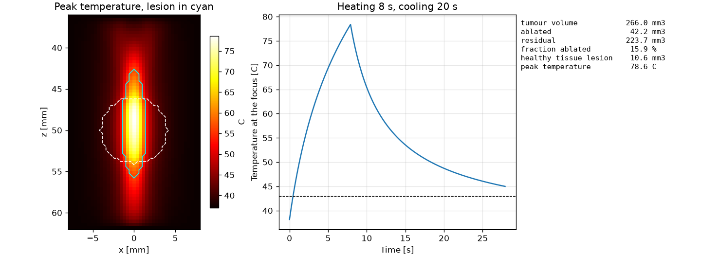
"""Thermal ablation of a spherical tumour with a focused bowl.

A 1 MHz bowl (20 mm aperture radius, 50 mm radius of curvature) heats a
tumour of 4 mm radius centred at the focus. The pressure field is the
Rayleigh integral in a homogeneous attenuating medium, scaled to a focal
amplitude of 3 MPa and treated as linear. The source is on for 8 s and the
tissue then cools for 20 s. The Pennes equation is solved in 3-D and the
lesion is the region with CEM43 of 240 min or more.

The tissue and tumour values below are generic numbers for the example and
not measured data.
"""

import matplotlib.pyplot as plt
import numpy as np

import sonosk as sk
import sonosk.plot as splt
from sonosk import field, phantom, thermal, transducer

F = 1e6
A = 20e-3
ROC = 50e-3
P_FOCUS = 3e6
TISSUE = sk.Material("tissue", 1540, 1050, alpha0=0.5, k=0.5, cp=3600, perfusion=0.5)
TUMOUR = sk.Material("tumour", 1540, 1050, alpha0=0.7, k=0.5, cp=3600, perfusion=0.3)


def _axisymmetric_field(r_max, z0, z1, h):
    """|p| of the bowl on an (r, z) grid; the bowl field is symmetric about z."""
    src = transducer.bowl(A, ROC, dx=TISSUE.c / F / 4)
    r = np.arange(0, r_max + h, h)
    z = np.arange(z0, z1 + h, h)
    rr, zz = np.meshgrid(r, z, indexing="ij")
    pts = np.stack([rr.ravel(), 0 * rr.ravel(), zz.ravel()], 1)
    p = np.abs(field.rayleigh(src, pts, F, TISSUE.c, alpha0=TISSUE.alpha0)).reshape(rr.shape)
    return r, z, p


def _interp_rz(r, z, p, R, Z):
    # bilinear interpolation of p(r, z) at the points (R, Z)
    fr = np.clip((R - r[0]) / (r[1] - r[0]), 0, r.size - 1.001)
    fz = np.clip((Z - z[0]) / (z[1] - z[0]), 0, z.size - 1.001)
    i, j = fr.astype(int), fz.astype(int)
    a, b = fr - i, fz - j
    return ((1 - a) * (1 - b) * p[i, j] + a * (1 - b) * p[i + 1, j]
            + (1 - a) * b * p[i, j + 1] + a * b * p[i + 1, j + 1])


def compute():
    g = sk.Grid.centered((41, 41, 66), 0.4e-3, depth_start=36e-3)
    x, y, z = g.mesh()
    lab = phantom.paint(np.zeros(g.shape, int), phantom.sphere(g, (0, 0, ROC), 4e-3), 1)
    med = sk.Medium(g, lab, [TISSUE, TUMOUR])

    r, zr, pr = _axisymmetric_field(np.hypot(*g.extent[:2]) / 2 + 1e-3, 35e-3, 63e-3, 0.2e-3)
    p = _interp_rz(r, zr, pr, np.hypot(x, y), z)
    p *= P_FOCUS / p.max()
    q = thermal.heat_source(p, med.attenuation(F), med.rho, med.c)

    on = 8.0
    res = thermal.bioheat(med, q, duration=28.0, schedule=lambda t: 1.0 if t < on else 0.0,
                          probe=[tuple(np.array(g.shape) // 2)])
    rep = thermal.treatment_report(res.lesion(), med, "tumour")
    return g, med, res, rep


def figure():
    g, med, res, rep = compute()
    xg, yg, zg = g.axes()
    j = g.shape[1] // 2
    fig, ax = plt.subplots(1, 3, figsize=(12, 4.4), constrained_layout=True,
                           gridspec_kw={"width_ratios": [1, 1.2, 0.9]})
    h = splt.temperature_map(res.T_max[:, j, :], xg, zg, ax=ax[0], lesion=res.lesion()[:, j, :],
                             title="Peak temperature, lesion in cyan")
    ax[0].contour(xg * 1e3, zg * 1e3, med.mask("tumour")[:, j, :].T.astype(float), levels=[0.5],
                  colors="white", linestyles="--", linewidths=1.0)
    fig.colorbar(h, ax=ax[0], shrink=0.8, label="C")

    t = np.arange(res.probe.shape[0]) * res.dt
    ax[1].plot(t, res.probe[:, 0])
    ax[1].axhline(43, color="k", lw=0.8, ls="--")
    ax[1].set_xlabel("Time [s]")
    ax[1].set_ylabel("Temperature at the focus [C]")
    ax[1].set_title("Heating 8 s, cooling 20 s")
    ax[1].grid(alpha=0.3)

    mm3 = 1e9
    rows = [f"{'tumour volume':<22s}{rep['target_volume'] * mm3:7.1f} mm3",
            f"{'ablated':<22s}{rep['ablated'] * mm3:7.1f} mm3",
            f"{'residual':<22s}{rep['residual'] * mm3:7.1f} mm3",
            f"{'fraction ablated':<22s}{100 * rep['fraction_ablated']:7.1f} %",
            f"{'healthy tissue lesion':<22s}{rep['healthy_damaged'] * mm3:7.1f} mm3",
            f"{'peak temperature':<22s}{res.T_max.max():7.1f} C"]
    ax[2].axis("off")
    ax[2].text(0.0, 0.98, "\n".join(rows), family="monospace", va="top", fontsize=9)
    return fig


if __name__ == "__main__":
    g, med, res, rep = compute()
    print(f"peak temperature {res.T_max.max():.1f} C, time step {res.dt:.3f} s")
    for k, v in rep.items():
        print(k, v)
    figure()
    plt.show()

Field of a focused bowl

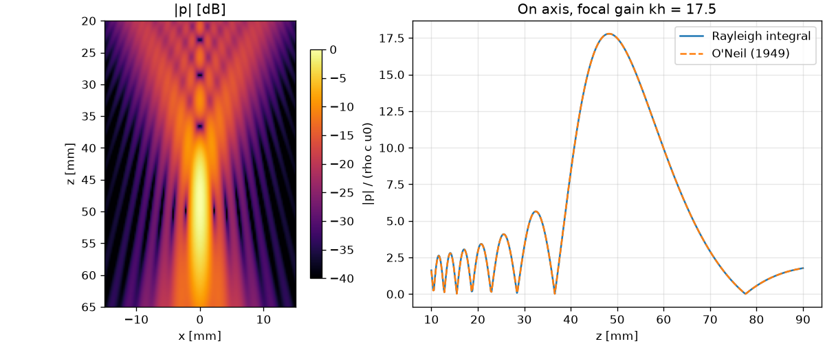
"""Pressure field of a focused bowl and comparison with O'Neil's solution.

A 1 MHz bowl with 20 mm aperture radius and 50 mm radius of curvature in
water. Left: field amplitude in the x-z plane from the Rayleigh integral.
Right: on-axis amplitude against the closed-form result.
"""

import matplotlib.pyplot as plt
import numpy as np

import sonosk as sk
import sonosk.plot as splt
from sonosk import analytic, field, transducer

F = 1e6
C = 1500.0
A = 20e-3
ROC = 50e-3


def compute():
    src = transducer.bowl(A, ROC, dx=C / F / 6)
    g = sk.Grid.centered((121, 181), 0.25e-3, depth_start=20e-3)
    p = field.rayleigh_grid(src, g, F, C)
    z = np.linspace(10e-3, 90e-3, 600)
    pz = np.abs(field.rayleigh(src, np.stack([0 * z, 0 * z, z], 1), F, C))
    return g, p, z, pz, analytic.bowl_axial(z, A, ROC, F, C)


def figure():
    g, p, z, pz, pa = compute()
    x, zz = g.axes()
    fig, ax = plt.subplots(1, 2, figsize=(10, 4.2), constrained_layout=True,
                           gridspec_kw={"width_ratios": [1, 1.4]})
    h = splt.field_map(p, x, zz, ax=ax[0], title="|p| [dB]")
    fig.colorbar(h, ax=ax[0], shrink=0.8)
    ax[1].plot(z * 1e3, pz, label="Rayleigh integral")
    ax[1].plot(z * 1e3, pa, "--", label="O'Neil (1949)")
    ax[1].set_xlabel("z [mm]")
    ax[1].set_ylabel("|p| / (rho c u0)")
    ax[1].set_title(f"On axis, focal gain kh = {analytic.focal_gain(A, ROC, F, C):.1f}")
    ax[1].legend()
    ax[1].grid(alpha=0.3)
    return fig


if __name__ == "__main__":
    figure()
    plt.show()

Linear array beams

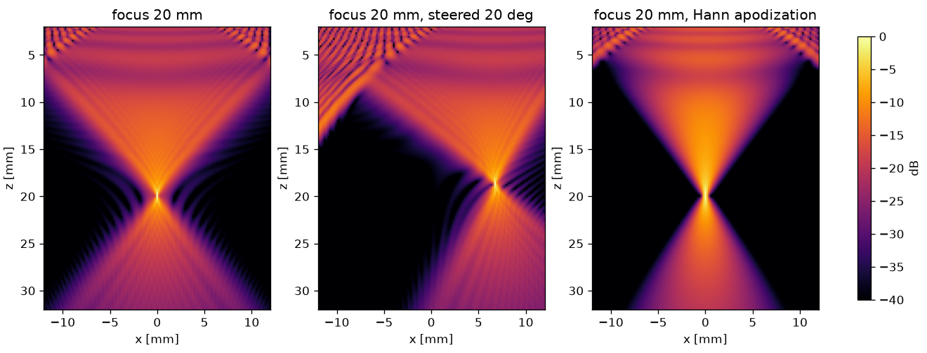
"""CW beams of a linear array: focused, focused and steered, and with a
Hann apodization.

128 elements, 0.3 mm pitch, 5 mm high with a 20 mm elevation lens, at
5 MHz in a medium with 1540 m/s and 0.5 dB/(cm MHz). Field amplitude in
the x-z plane, normalised in each panel.
"""

import matplotlib.pyplot as plt
import numpy as np

import sonosk as sk
import sonosk.plot as splt
from sonosk import field, transducer

F = 5e6
C = 1540.0


def compute():
    arr = transducer.linear_array(128, 0.3e-3, height=5e-3, elev_focus=20e-3, dx=0.15e-3)
    g = sk.Grid.centered((121, 151), 0.2e-3, depth_start=2e-3)
    out = []
    arr.focus((0, 0, 20e-3), C)
    out.append(("focus 20 mm", field.rayleigh_grid(arr, g, F, C, alpha0=0.5)))
    fp = 20e-3 * np.array([np.sin(np.deg2rad(20)), 0, np.cos(np.deg2rad(20))])
    arr.focus(fp, C)
    out.append(("focus 20 mm, steered 20 deg", field.rayleigh_grid(arr, g, F, C, alpha0=0.5)))
    arr.focus((0, 0, 20e-3), C).set_apodization(transducer.apodization(128, "hann"))
    out.append(("focus 20 mm, Hann apodization", field.rayleigh_grid(arr, g, F, C, alpha0=0.5)))
    return g, out


def figure():
    g, out = compute()
    x, z = g.axes()
    fig, ax = plt.subplots(1, 3, figsize=(11, 4.2), constrained_layout=True)
    for a, (title, p) in zip(ax, out):
        h = splt.field_map(p, x, z, ax=a, title=title, dynamic_range=40)
    fig.colorbar(h, ax=ax, shrink=0.8, label="dB")
    return fig


if __name__ == "__main__":
    figure()
    plt.show()

Line-focus source

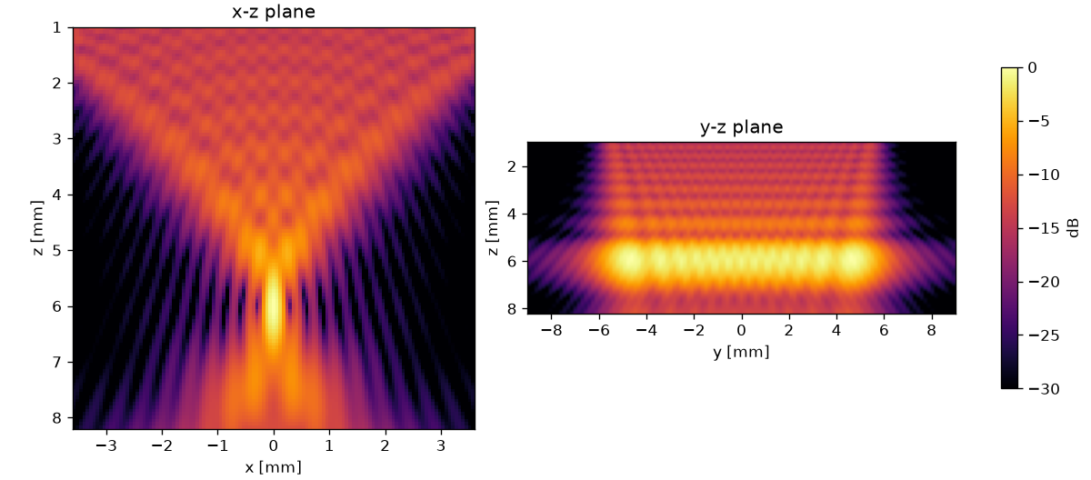
"""Field of a cylindrically focused source, the geometry of line-focused
aesthetic HIFU transducers.

A 4 MHz source with 8 mm chord, 12 mm length and 6 mm radius of curvature
focuses to a line 6 mm under the face. The values are an example, not the
data of a commercial device. Left: x-z plane through the middle of the
line. Right: y-z plane through the focus line.
"""

import matplotlib.pyplot as plt
import numpy as np

import sonosk as sk
import sonosk.plot as splt
from sonosk import field, transducer

F = 4e6
C = 1540.0


def compute():
    src = transducer.cylindrical(8e-3, 12e-3, 6e-3, dx=0.08e-3)
    gx = sk.Grid.centered((121, 121), 0.06e-3, depth_start=1e-3)
    pxz = field.rayleigh_grid(src, gx, F, C, alpha0=0.5)
    y = np.linspace(-9e-3, 9e-3, 121)
    z = gx.axis(1)
    yy, zz = np.meshgrid(y, z, indexing="ij")
    pyz = field.rayleigh(src, np.stack([0 * yy.ravel(), yy.ravel(), zz.ravel()], 1),
                         F, C, alpha0=0.5).reshape(yy.shape)
    return gx, pxz, y, pyz


def figure():
    gx, pxz, y, pyz = compute()
    x, z = gx.axes()
    fig, ax = plt.subplots(1, 2, figsize=(10, 4.4), constrained_layout=True)
    splt.field_map(pxz, x, z, ax=ax[0], title="x-z plane", dynamic_range=30)
    h = splt.field_map(pyz, y, z, ax=ax[1], title="y-z plane", dynamic_range=30)
    ax[1].set_xlabel("y [mm]")
    fig.colorbar(h, ax=ax, shrink=0.8, label="dB")
    return fig


if __name__ == "__main__":
    figure()
    plt.show()

Element design with the Mason model

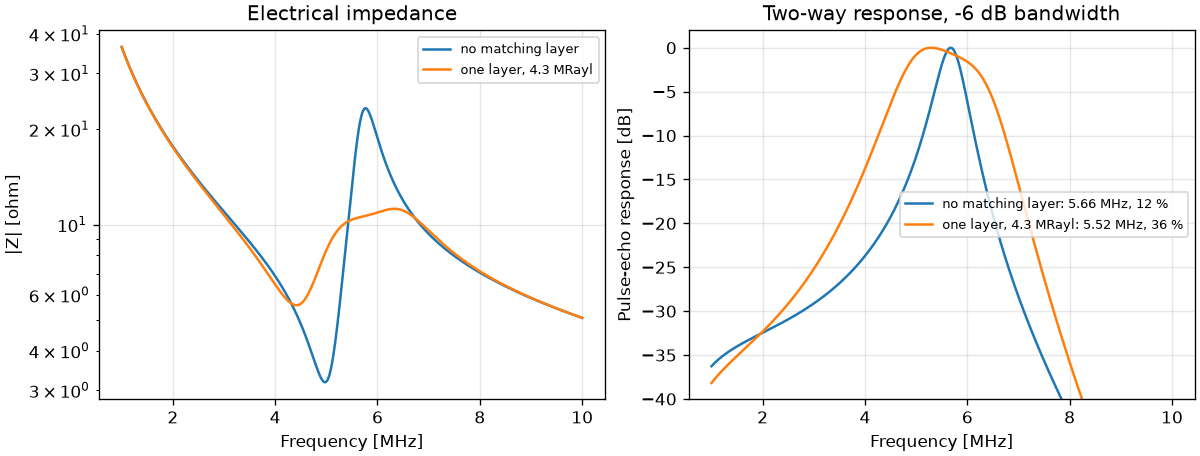
"""Design of a 5.7 MHz thickness-mode element with the Mason model.

A 0.4 mm piezoceramic plate (10 mm x 10 mm) on a 3 MRayl backing radiates
into water, without and with a quarter-wave matching layer whose
impedance follows Desilets et al. (1978). The plate constants are typical
of a soft PZT and are only an example; use the data sheet of the material
you build with.
"""

import matplotlib.pyplot as plt
import numpy as np

from sonosk import stack

PLATE = stack.Piezo(thickness=0.4e-3, c=4560.0, rho=7500.0, kt=0.5, eps_r=1470.0,
                    area=1e-4)
F = np.linspace(1e6, 10e6, 2000)


def compute():
    plain = stack.Stack(PLATE, backing=3e6, load=1.5e6)
    zm = stack.matching_impedance(PLATE.impedance, 1.5e6)
    cm = 2500.0
    lay = stack.Layer(stack.quarter_wave(cm, PLATE.f_half_wave), cm, zm / cm)
    matched = stack.Stack(PLATE, backing=3e6, layers=[lay], load=1.5e6)
    return {"no matching layer": plain, f"one layer, {zm / 1e6:.1f} MRayl": matched}


def figure():
    stacks = compute()
    fig, ax = plt.subplots(1, 2, figsize=(10, 3.8), constrained_layout=True)
    for name, s in stacks.items():
        z = s.impedance(F)
        ax[0].semilogy(F / 1e6, np.abs(z), label=name)
        h = s.pulse_echo(F)
        fc, bw = stack.bandwidth(F, h)
        ax[1].plot(F / 1e6, 20 * np.log10(np.abs(h)),
                   label=f"{name}: {fc / 1e6:.2f} MHz, {100 * bw:.0f} %")
    ax[0].set_xlabel("Frequency [MHz]")
    ax[0].set_ylabel("|Z| [ohm]")
    ax[0].set_title("Electrical impedance")
    ax[1].set_xlabel("Frequency [MHz]")
    ax[1].set_ylabel("Pulse-echo response [dB]")
    ax[1].set_ylim(-40, 2)
    ax[1].set_title("Two-way response, -6 dB bandwidth")
    for a in ax:
        a.grid(alpha=0.3)
        a.legend(fontsize=8)
    return fig


if __name__ == "__main__":
    for name, s in compute().items():
        fc, bw = stack.bandwidth(F, s.pulse_echo(F))
        print(f"{name}: centre {fc / 1e6:.2f} MHz, bandwidth {100 * bw:.0f} %")
    figure()
    plt.show()

Mechanical index

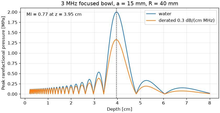
"""Mechanical index of a focused bowl from its on-axis pressure.

A 3 MHz bowl, 15 mm aperture radius and 40 mm radius of curvature, is
driven so that the peak pressure in water is 2 MPa. The on-axis field is
the O'Neil solution, derated at 0.3 dB/(cm MHz).
"""

import matplotlib.pyplot as plt
import numpy as np

from sonosk import analytic, safety

F = 3e6
A = 15e-3
ROC = 40e-3
P_PEAK = 2.0  # MPa in water


def compute():
    z = np.linspace(2e-3, 80e-3, 2000)
    p = analytic.bowl_axial(z, A, ROC, F)
    pr = P_PEAK * p / p.max()
    z_cm = z * 100.0
    mi, z_sp = safety.mechanical_index(z_cm, pr, F / 1e6)
    pr3 = safety.derate(pr, F / 1e6, z_cm)
    return z_cm, pr, pr3, mi, z_sp


def figure():
    z_cm, pr, pr3, mi, z_sp = compute()

    fig, ax = plt.subplots(figsize=(7, 3.6), constrained_layout=True)
    ax.plot(z_cm, pr, label="water")
    ax.plot(z_cm, pr3, label="derated 0.3 dB/(cm MHz)")
    ax.axvline(z_sp, color="k", lw=0.8, ls="--")
    ax.text(0.03, 0.95, f"MI = {mi:.2f} at z = {z_sp:.2f} cm", transform=ax.transAxes, va="top")
    ax.set_xlabel("Depth [cm]")
    ax.set_ylabel("Peak rarefactional pressure [MPa]")
    ax.set_title("3 MHz focused bowl, a = 15 mm, R = 40 mm")
    ax.legend(loc="upper right")
    ax.grid(alpha=0.3)
    return fig


if __name__ == "__main__":
    z_cm, pr, pr3, mi, z_sp = compute()
    print(f"MI = {mi:.3f} at z = {z_sp:.2f} cm")
    print(safety.check_limits(mi=mi, ispta3=300.0))
    figure()
    plt.show()

Water properties

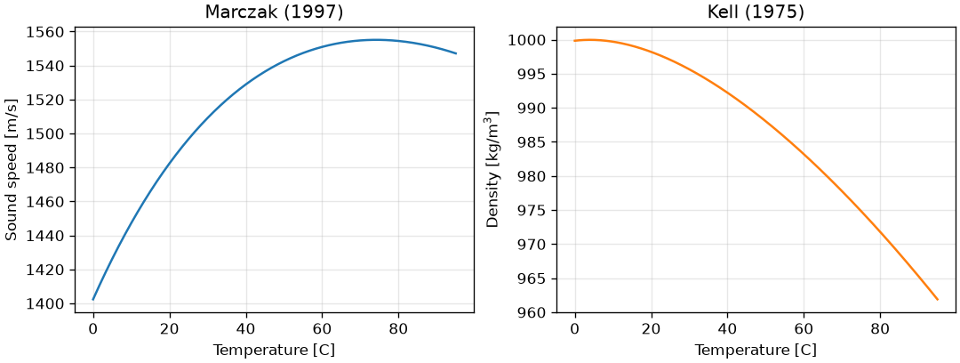
"""Sound speed and density of water between 0 and 95 C."""

import matplotlib.pyplot as plt
import numpy as np

from sonosk import water


def figure():
    t = np.linspace(0.0, 95.0, 400)

    fig, ax = plt.subplots(1, 2, figsize=(9, 3.4), constrained_layout=True)
    ax[0].plot(t, water.sound_speed(t), color="C0")
    ax[0].set_xlabel("Temperature [C]")
    ax[0].set_ylabel("Sound speed [m/s]")
    ax[0].set_title("Marczak (1997)")

    ax[1].plot(t, water.density(t), color="C1")
    ax[1].set_xlabel("Temperature [C]")
    ax[1].set_ylabel("Density [kg/m$^3$]")
    ax[1].set_title("Kell (1975)")

    for a in ax:
        a.grid(alpha=0.3)
    return fig


if __name__ == "__main__":
    figure()
    plt.show()