Probe design¶

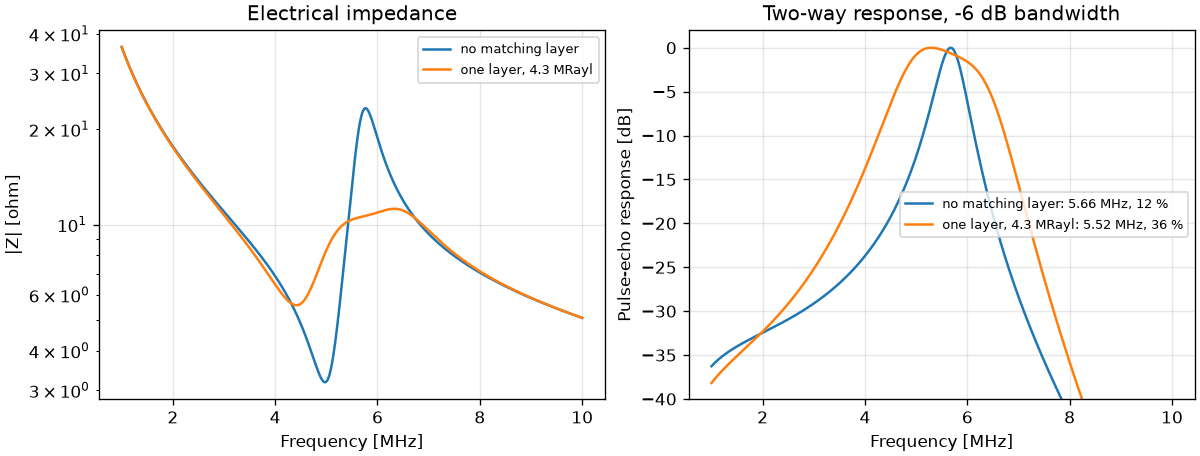
sonosk.stack models one element of a probe in thickness mode, so the effect of the piezoelectric material, the backing and the matching layers can be seen before anything is built.

Model¶

The plate is described by the Mason equivalent circuit. Backing and load are semi-infinite media given by their acoustic impedance in Rayl. Matching layers and a lens are transmission lines, with attenuation if alpha0 is set. For an unloaded plate the model reduces to the known closed form

\[ Z = \frac{1}{j\omega C_0}\left(1 - k_t^2 \frac{\tan(\beta d / 2)}{\beta d / 2}\right), \]

and with lossless layers the electrical power going in equals the acoustic power going out into backing and load (see Validation).

Building a stack¶

from sonosk import stack

plate = stack.Piezo(thickness=0.4e-3, c=4560.0, rho=7500.0, kt=0.5,
                    eps_r=1470.0, area=1e-4)
plate.f_half_wave                     # c / (2 d)
plate.c0                              # clamped capacitance

z_m = stack.matching_impedance(plate.impedance, 1.5e6)        # Desilets et al.
layer = stack.Layer(stack.quarter_wave(2500.0, plate.f_half_wave), 2500.0, z_m / 2500.0)
s = stack.Stack(plate, backing=3e6, layers=[layer], load=1.5e6)

Piezo.c is the stiffened longitudinal sound speed of the plate and eps_r the clamped relative permittivity \(\varepsilon_{33}^S/\varepsilon_0\). Take both, with kt and rho, from the data sheet of the material. The numbers above are only an example.

Responses¶

f = np.linspace(1e6, 10e6, 2000)
s.impedance(f)                 # electrical input impedance [ohm]
s.transmit(f, r_source=50.0)   # pressure in the load per volt [Pa/V]
h = s.pulse_echo(f)            # two-way response, normalised
fc, bw = stack.bandwidth(f, h) # centre frequency and -6 dB fractional bandwidth
s.power_balance(f)             # electrical and acoustic power for 1 A

fc and bw can be passed to imaging.Pulse to image with the designed element.

Electrical impedance and pulse-echo response with and without a matching layer

Limits of this release¶

The model is one-dimensional. Lateral modes, kerf coupling between elements and the shape of the lens need finite-element models and are not included.

References¶

Mason W.P. Electromechanical Transducers and Wave Filters, 2nd ed. Van Nostrand, 1948.

Kino G.S. Acoustic Waves: Devices, Imaging, and Analog Signal Processing. Prentice-Hall, 1987.

Desilets C.S., Fraser J.D., Kino G.S. The design of efficient broad-band piezoelectric transducers. IEEE Trans. Sonics Ultrason. 25(3):115-125, 1978.