Pressure fields

sonosk.field computes continuous-wave (CW) pressure fields. The time convention is \(e^{j\omega t}\).

Rayleigh integral

For a source with normal velocity amplitude \(u_0\), the pressure at a point \(\mathbf{r}\) is

\[ \frac{p(\mathbf{r})}{\rho c u_0} = \frac{jk}{2\pi} \sum_n w_n A_n \frac{e^{-(jk + \alpha) R_n}}{R_n}, \]

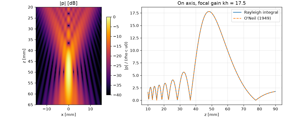
where \(A_n\) is the area of patch \(n\), \(R_n\) its distance to the point, \(w_n\) its complex weight from the apodization and the firing delay, and \(\alpha\) the amplitude attenuation of a homogeneous medium in Np/m. For a curved source each patch is treated as part of a baffled plane, the usual approximation behind the O’Neil solution.

import numpy as np
import sonosk as sk
from sonosk import field, transducer

bowl = transducer.bowl(20e-3, 50e-3, dx=0.25e-3)
pts = np.array([[0, 0, 45e-3], [0, 0, 50e-3], [1e-3, 0, 50e-3]])
p = field.rayleigh(bowl, pts, f=1e6, c=1500.0)              # p / (rho c u0)

g = sk.Grid.centered((121, 181), 0.25e-3, depth_start=20e-3)
pg = field.rayleigh_grid(bowl, g, f=1e6, c=1500.0, alpha0=0.5)

rayleigh_grid evaluates a 1-D grid on the z axis, a 2-D grid in the x-z plane (at plane_y) and a 3-D grid everywhere. The cost grows with the number of points times the number of patches; max_pairs limits the memory used at once.

Angular spectrum

When the field is known on a plane, the angular spectrum method carries it to other depths with fast Fourier transforms:

x = np.arange(-30e-3, 30e-3, 0.5e-3)
X, Y = np.meshgrid(x, x, indexing="ij")
plane = field.rayleigh(bowl, np.stack([X.ravel(), Y.ravel(), np.full(X.size, 5e-3)], 1),
                       1e6, 1500.0).reshape(X.shape)
vol = field.angular_spectrum(plane, dx=0.5e-3, f=1e6, z=[10e-3, 20e-3, 30e-3], c=1500.0)

A 1-D input is a field that does not change along y, which turns the problem into a 2-D one. Use pad to reduce wrap-around from the periodic transform, and a plane large enough to hold the beam.

Physical units

The solvers return \(p / (\rho c u_0)\). scale_to_pressure gives pascals from the surface velocity, or from the acoustic power of a uniform plane source, and intensity gives the plane-wave intensity \(|p|^2 / (2 \rho c)\).

p_pa = field.scale_to_pressure(p, rho=1000.0, c=1500.0, u0=0.05)
I = field.intensity(p_pa, rho=1000.0, c=1500.0)                # W/m^2

Limits of this release

The medium is homogeneous: one sound speed and one attenuation for the whole path. Refraction and reflection at tissue layers, and nonlinear propagation at high amplitude, need the full-wave and nonlinear solvers on the Roadmap.

References

O’Neil H.T. Theory of focusing radiators. J. Acoust. Soc. Am. 21(5):516-526, 1949.

Zeng X., McGough R.J. Evaluation of the angular spectrum approach for simulations of near-field pressures. J. Acoust. Soc. Am. 123(1):68-76, 2008.