Imaging¶

sonosk.imaging simulates the echo signals of an array and forms B-mode images from them.

The forward model¶

The model is linear (first-order Born scattering) in a homogeneous medium of sound speed \(c\):

the transmit wave comes from a virtual source: a plane wave with a steering angle, a diverging wave from a point behind the array, or a wave focused on a point in front of it;
each receive element is a point receiver with the directivity of a rectangular element in a soft baffle, \(\mathrm{sinc}(w \sin\theta / \lambda)\cos\theta\);
spreading is \(1/R\) on the receive path, and from the virtual source for a diverging wave; attenuation is applied at the centre frequency along both paths.

Each scatterer returns a copy of the two-way pulse delayed by its travel time. The echoes are placed on a time axis four times finer than the output rate, convolved with the pulse and decimated. The signals are kept in analytic (complex) form, so the envelope of an image is its modulus.

Pulse¶

from sonosk import imaging

pulse = imaging.Pulse(f0=5e6, bandwidth=0.6)    # 60 % -6 dB bandwidth

The pulse is a Gaussian-modulated sinusoid and stands for the whole two-way response: excitation, transmit and receive. The axial resolution follows from it (see Validation). The response of a designed stack can be used to choose f0 and bandwidth (see Probe design).

Transmits¶

tx = imaging.Transmit.plane(angle=0.0)
tx = imaging.Transmit.diverging(source=(0, 0, -10e-3))
tx = imaging.Transmit.focused(point=(0, 0, 30e-3))
angles = imaging.plane_wave_angles(9, span=np.deg2rad(24))

A plane wave insonifies the strip in front of the aperture. Diverging waves suit phased and convex arrays with a wide sector.

Simulation and beamforming¶

rf, fs = imaging.simulate(probe, tx, pos, amp, pulse, c=1540.0, alpha0=0.5)
img = imaging.beamform(rf, fs, probe, tx, x, z, c=1540.0, f_number=1.5)

rf has one row per element. beamform is delay-and-sum on the grid x by z (in the x-z plane), with a receive aperture set by f_number and a Hann window across it. compound adds the images of several transmits:

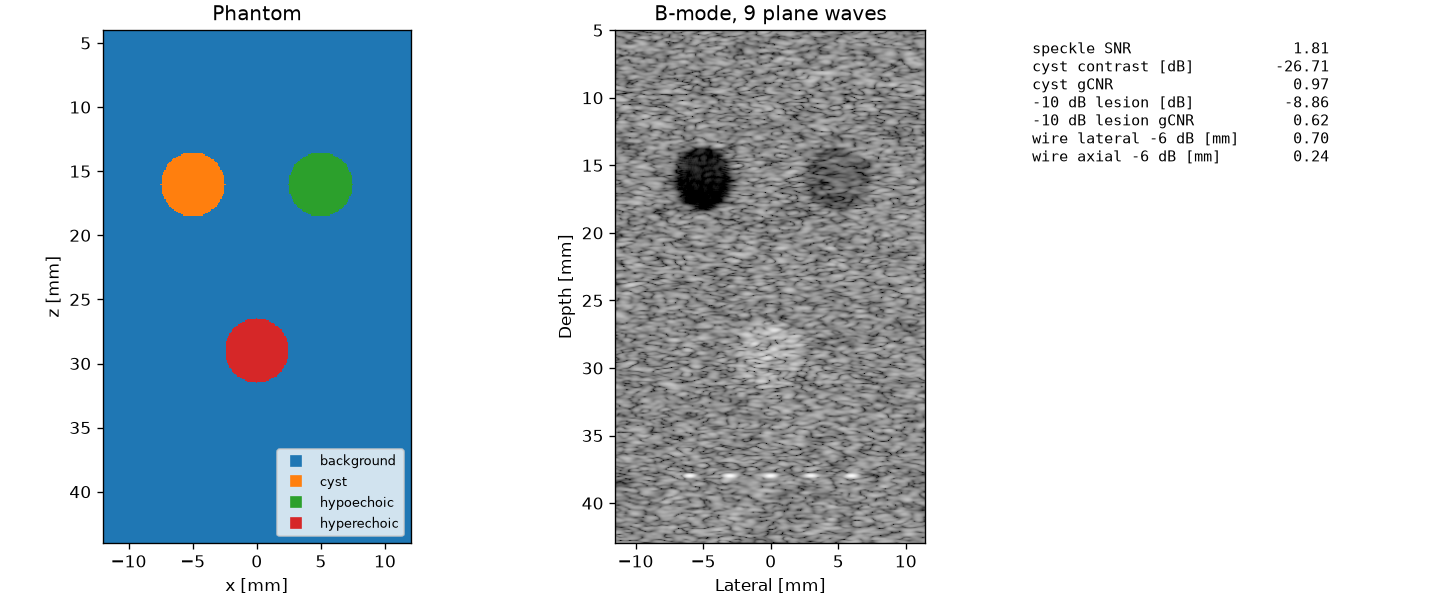
transmits = [imaging.Transmit.plane(a) for a in angles]
rfs = [imaging.simulate(probe, t, pos, amp, pulse)[0] for t in transmits]
img = imaging.compound(rfs, fs, probe, transmits, x, z)
db = imaging.log_compress(img, dynamic_range=60)

Phantom, compounded B-mode image and quality measures

Run time¶

The simulation costs about elements times scatterers operations per transmit. A 128-element array with 35 000 scatterers takes about half a second per transmit on a laptop; beamforming a 300 by 500 pixel image takes about one second per transmit.

Limits of this release¶

The medium is homogeneous in sound speed. Echoes from layers with a different speed are placed at the right amplitude but without the refraction and aberration a real fat layer causes; these need the full-wave solver on the Roadmap. The image plane is 2-D; volume imaging with matrix arrays is planned for version 0.3.

References¶

Montaldo G., Tanter M., Bercoff J., Benech N., Fink M. Coherent plane-wave compounding for very high frame rate ultrasonography and transient elastography. IEEE Trans. Ultrason. Ferroelectr. Freq. Control 56(3):489-506, 2009.

Garcia D. SIMUS: an open-source simulator for medical ultrasound imaging. Part I: theory & examples. Comput. Methods Programs Biomed. 218:106726, 2022.