Therapy

sonosk.thermal follows a therapeutic exposure from the pressure field to the lesion: heat source, temperature, thermal dose and the volumes treated and spared.

Heat source

For a CW field with pressure amplitude \(p\), the absorbed power density is

\[ Q = 2\alpha I = \frac{\alpha |p|^2}{\rho c}, \]

with \(\alpha\) the amplitude absorption coefficient in Np/m. When only the attenuation is known it is often used in place of the absorption, which overestimates heating in strongly scattering tissue.

from sonosk import field, thermal

p = field.rayleigh_grid(src, grid, f, c, alpha0)       # p / (rho c u0)
p = 3e6 * np.abs(p) / np.abs(p).max()                   # scale, here to 3 MPa
q = thermal.heat_source(p, medium.attenuation(f), medium.rho, medium.c)

Bioheat equation

The temperature follows the Pennes equation

\[ \rho c_p \frac{\partial T}{\partial t} = \nabla\cdot(k \nabla T) + w_b c_b (T_a - T) + Q, \]

with \(w_b\) the perfusion in kg/(m³ s), \(c_b\) the specific heat of blood and \(T_a\) the arterial temperature. It is solved with an explicit finite difference scheme on the grid of the medium, in 1, 2 or 3 dimensions. The outer boundary is held at the initial temperature, so the grid must be large enough that the heated region stays away from it.

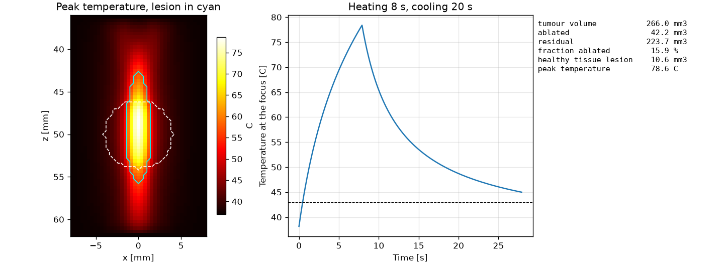
res = thermal.bioheat(medium, q, duration=28.0,
                      schedule=lambda t: 1.0 if t < 8.0 else 0.0,
                      T0=37.0, snapshots=[8.0, 28.0], probe=[(20, 20, 32)])
res.T_max        # highest temperature at each point
res.T            # fields at the snapshot times
res.probe        # temperature history at the probe points
res.dt           # time step used

schedule(t) gives the power fraction at time t, so pulsed and repeated sonications can be modelled. The time step is 0.9 of the stability limit and at most max_dt (0.1 s); it must be short against the on and off times of the schedule.

Thermal dose and lesion

\[\begin{split} \mathrm{CEM}_{43} = \sum \Delta t\, R^{43 - T},\qquad R = \begin{cases} 0.5 & T \ge 43\,^\circ\mathrm{C}\\ 0.25 & T < 43\,^\circ\mathrm{C}\end{cases} \end{split}\]

with \(\Delta t\) in minutes (Sapareto and Dewey 1984). The solver adds up the dose at every step. A dose of 240 min is the threshold commonly used for thermal necrosis in soft tissue:

lesion = res.lesion(threshold=240.0)
thermal.cem43(T_history, dt)       # dose of any temperature history

Treatment report

rep = thermal.treatment_report(lesion, medium, target="tumour")
rep["fraction_ablated"], rep["residual"], rep["healthy_damaged"]

The report gives the target volume, the ablated and residual target, the damaged volume outside the target and the damaged volume of every material.

Limits of this release

The properties do not change with temperature, and perfusion stays on in the lesion. Arrhenius damage, temperature-dependent properties and perfusion shutdown are planned for version 0.2; nonlinear heating at high pressure needs the nonlinear solver planned for version 0.3.

References

Pennes H.H. Analysis of tissue and arterial blood temperatures in the resting human forearm. J. Appl. Physiol. 1(2):93-122, 1948.

Sapareto S.A., Dewey W.C. Thermal dose determination in cancer therapy. Int. J. Radiat. Oncol. Biol. Phys. 10(6):787-800, 1984.