Benchmarks

The tests on the Validation page compare each solver with a closed-form result. This page adds convergence studies, which show how the error falls as the grid gets finer, and a comparison of the full-wave solver with k-Wave on a shared case. The numbers come from benchmarks/run_benchmarks.py and benchmarks/kwave_comparison.py in the repository, which write them to benchmarks/results.json and benchmarks/kwave_comparison.json together with the software versions (sonosk.run_info()), so that each release can be compared with the one before. The studies themselves are in sonosk.benchmarks.

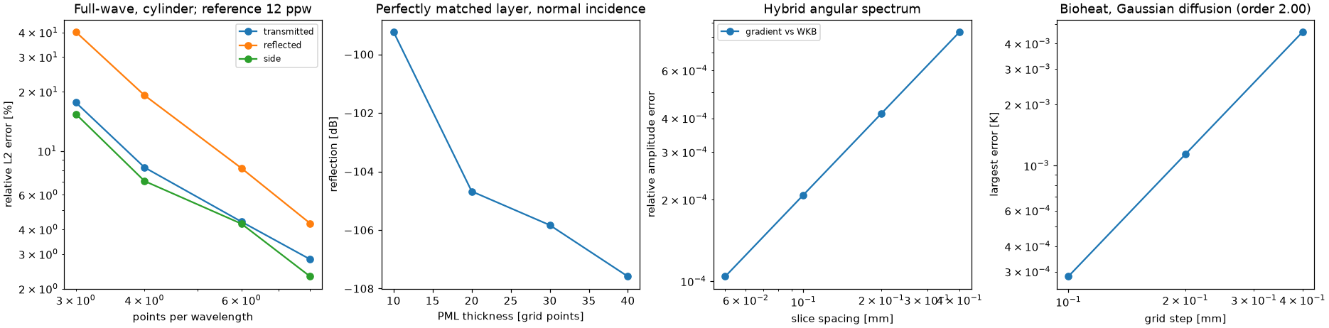
Full-wave solver against grid resolution

A plane wave (three-cycle burst at 1 MHz) from a line source meets a fluid cylinder of 2 wavelengths radius (1650 m/s, 1150 kg/m³) in water. The pressure is recorded at a transmitted, a reflected and a side point, all on multiples of the wavelength so that they fall on grid points of every grid, and compared with the run at 12 points per wavelength.

Points per wavelength	3	4	6	8
Transmitted, relative L2 error	17.6 %	8.2 %	4.4 %	2.8 %
Reflected	40.2 %	19.2 %	8.2 %	4.3 %
Side	15.4 %	7.0 %	4.3 %	2.3 %

The error comes from the staircase of the cylinder on the grid; in a homogeneous medium the scheme is exact. Weak echoes from sharp interfaces need the most points per wavelength.

Perfectly matched layer

A pulse at normal incidence in 1-D; the reflected amplitude relative to the incident one is -99 dB with 10 points of layer, -105 dB with 20, -106 dB with 30 and -108 dB with 40 (absorption 2 Np per point).

Hybrid angular spectrum against slice spacing

Through a linear density gradient (1000 to 1500 kg/m³ over 10 mm) the amplitude converges to \(\sqrt{Z_2/Z_1}\) with first-order error: 0.083 % at 0.4 mm, 0.042 % at 0.2 mm, 0.021 % at 0.1 mm and 0.010 % at 0.05 mm. Through a sharp step of the same size it equals \(2Z_2/(Z_1+Z_2)\) to rounding error for every slice spacing.

Bioheat solver

A Gaussian temperature rise of 10 K and 1 mm width spreads by conduction for 20 s and is compared with the analytic solution. With the time step a fixed fraction of the stability limit, the largest error is 4.6 mK at 0.4 mm, 1.1 mK at 0.2 mm and 0.28 mK at 0.1 mm: second order in space and time together.

Error of a single power-law exponent

With the default single exponent of the full-wave solver (here the median 1.6 of seven tissues, with f_ref = 3 MHz), the attenuation of each tissue is exact at 3 MHz and off elsewhere by the factor \((f/f_\mathrm{ref})^{y_\mathrm{grid} - y_\mathrm{tissue}}\):

Tissue	y	Attenuation ratio at 1.5 MHz	at 6 MHz	Phase speed error at 1.5 / 6 MHz [m/s]
fat	1.00	0.66	1.52	+0.63 / -0.23
muscle	1.08	0.70	1.43	+0.53 / -0.22
prostate	1.10	0.71	1.41	+0.66 / -0.30
myometrium	1.60	1.00	1.00	0 / 0
fibroid	1.65	1.04	0.97	-0.08 / +0.08
dermis	1.69	1.06	0.94	-0.11 / +0.12
cervix	2.09	1.40	0.71	-1.01 / +1.68

y="tissue" in fullwave.simulate gives every tissue its own exponent; in the two-slab test of the test suite this brought the error of the measured attenuation from 49 % down to 2.7 % over 1.5 to 4.5 MHz.

Comparison with k-Wave

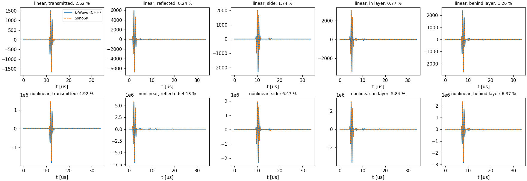
Both codes run the same 2-D problem: a 216 by 216 grid at 0.1 mm with the same time step and a perfectly matched layer of 20 points outside the grid; an absorbing background (0.5 dB/(cm MHz^1.5)) with a slow layer (1450 m/s) and a fast, dense cylinder (1600 m/s, 1100 kg/m³); a point source driven by a 1.5 MHz three-cycle burst. k-Wave runs through k-wave-python 0.6.2 with its compiled C++ binary, an implementation independent of SonoSK. After a shift of one time step, which comes from the different indexing of the source samples, the traces agree as follows:

Point	Relative L2 error, linear	Peak error, linear
reflected	0.24 %	0.01 %
in the layer	0.77 %	0.15 %
behind the layer	1.26 %	0.26 %
side	1.74 %	0.28 %
transmitted through the cylinder	2.62 %	0.47 %

In the nonlinear run (\(B/A\) = 6, a source strong enough for 1 to 7 MPa at the sensors) the nonlinear terms change the traces by 10 to 23 % against the scaled linear ones. There SonoSK and k-Wave agree to 4.1 to 6.5 % (relative L2) and 1.7 to 5.2 % in peak pressure. The difference is larger than in the linear case; the pressure next to the point source is very high in this run, and finding where the two codes part is an open item for version 0.3. In 1-D, the harmonics of SonoSK agree with the Fubini solution to 0.002 of the source amplitude (Validation page).

Each run took about 25 s with SonoSK and 26 to 48 s with the k-Wave binary (two CPU cores, including the file input and output of k-Wave).

The remaining differences grow with the path through the inclusions. The two codes differ in two documented details: the density on the staggered grid (k-Wave interpolates it spectrally, SonoSK averages neighbours), and the time at which the absorption term is evaluated (SonoSK extrapolates the divergence of the velocity to the time of the pressure).

Still to do

Comparisons of the fast imaging model with Field II or FOCUS, of the beamformers with the PICMUS data, and of fields and temperatures with measurements are planned for version 0.3.