Full-wave simulation

sonosk.fullwave solves the equations of nonlinear acoustics in a heterogeneous, absorbing fluid with a k-space pseudospectral method, in 1, 2 or 3 dimensions. It covers what the fast models leave out: refraction, reflection, diffraction, multiple scattering, power-law absorption with its dispersion, and the harmonics of nonlinear propagation.

Equations

The solver integrates the coupled first-order equations

\[ \frac{\partial \mathbf u}{\partial t} = -\frac{1}{\rho_0}\nabla p,\qquad \frac{\partial \rho}{\partial t} = -(2\rho + \rho_0)\,\nabla\cdot\mathbf u, \]

\[ p = c_0^2\left(\rho + \frac{B}{2A}\frac{\rho^2}{\rho_0} - L\rho\right), \qquad L = \tau\frac{\partial}{\partial t}(-\nabla^2)^{\frac{y}{2}-1} + \eta(-\nabla^2)^{\frac{y+1}{2}-1}, \]

with \(\tau = -2\alpha_0 c_0^{y-1}\) and \(\eta = 2\alpha_0 c_0^{y}\tan(\pi y/2)\), which give the attenuation \(\alpha_0 f^y\) and the dispersion that goes with it (Treeby and Cox 2010; Treeby et al. 2012). Spatial derivatives are computed with FFTs on a staggered grid and corrected by the k-space operator \(\mathrm{sinc}(c_\mathrm{ref} k \Delta t/2)\) (Tabei et al. 2002), which makes the scheme exact in a homogeneous medium: there two to three points per wavelength are enough. Sharp interfaces are staircased on the grid and need more: for a plane wave on a sharp cylinder the error of the transmitted trace is 8 % at 4 points per wavelength and 3 % at 8 (see Benchmarks). A perfectly matched layer is added outside the grid; it reflects less than -99 dB at normal incidence with 20 points.

The divergence of the velocity, known at half time steps, is extrapolated to the time of the pressure before it enters the absorption term. With the plain half-step lag the phase speed drifts from the Kramers-Kronig relation by about 1 m/s at 5 MHz (CFL number 0.3); with the extrapolation the drift is below 0.1 m/s.

Running a simulation

import sonosk as sk
from sonosk import fullwave as fw, tissues

g = sk.Grid((400, 500), 0.1e-3)
med = sk.Medium(g, labels, [tissues.material("fat"), tissues.material("muscle")])
src = fw.Source(index, fw.tone_burst(1e6, 3), weight=1e5)       # Pa
res = fw.simulate(med, src, t_end=60e-6, sensor=fw.Sensor(points),
                  nonlinear=True, f_ref=1e6, record_max=True, cw=[1e6, 2e6])
res.p           # pressure at the sensor points, one row per point
res.p_max       # largest pressure at every grid point
res.cw[2e6]     # complex amplitude of the second harmonic

Option	Meaning
nonlinear	include \(B/A\) and convective nonlinearity
absorbing	include power-law absorption and dispersion
y, f_ref	one exponent for the grid; each tissue keeps its own attenuation at f_ref, and medium.c is the phase speed at f_ref
cfl, dt	time step, default 0.3 of the stability step
pml, pml_alpha	thickness and strength of the absorbing layer
record_max, record_rms, cw	maps of peak, RMS and harmonic amplitudes
precision="single"	half the memory, about twice the speed with scipy
max_memory	refuse runs that need more memory [bytes]; memory_estimate() gives the need

The arguments are checked before the run. A CFL number above 0.5 gives a warning, because the scheme is exact only in a homogeneous medium, and the run stops with FloatingPointError if the pressure stops being finite.

Power-law exponents

By default the grid uses one exponent \(y\) (the median of the tissues) and each tissue keeps its own attenuation at f_ref. Away from f_ref the attenuation of a tissue is then off by the factor \((f/f_\mathrm{ref})^{y - y_\mathrm{tissue}}\), and its phase speed by a fraction of a metre per second to a few metres per second; fullwave.exponent_error() gives both. With y="tissue" every distinct exponent gets its own pair of fractional Laplacian operators, so each tissue follows its own power law at all frequencies; the cost grows by two inverse FFTs per extra exponent and time step. In a test with two slabs (\(y\) = 1.2 and 1.8) the attenuation measured inside the second slab from 1.5 to 4.5 MHz was within 2.7 % of its own law with y="tissue", and off by up to 49 % with a single exponent.

res = fw.simulate(med, src, t_end, f_ref=3e6, y="tissue")
ratio, dc = fw.exponent_error(alpha0=0.73, y_tissue=1.0, f=[1.5e6, 6e6],
                              f_ref=3e6, y_grid=1.6)

Sources are Source(index, signal, delay, weight, kind): grid points with a waveform, per-point delays and weights, as a pressure (mass) source or a velocity source. array_source(transducer, grid, signal) and array_sensor(transducer, grid) map the elements of a transducer to grid points.

Pulse-echo imaging

fullwave.pulse_echo(medium, array, transmit, pulse) fires the elements with the delays of an imaging.Transmit, records the echoes on the same elements and returns analytic signals in the time convention of sonosk.imaging, ready for imaging.beamform and imaging.compound. Speckle comes from phantom.fluctuations, small random variations of density (and of speed, unless speed=0) scaled by the echo level of each tissue.

By default the elements transmit and receive a normal particle velocity (directional=True), which gives them the \(\cos\theta\) directivity of a baffled element. Omnidirectional pressure points hear the transmitted wave running along the face of the array, in 2-D above all, where the Green’s function has a long tail; that signal beamforms into a bright X over the near field. A receive band-pass filter (band, in multiples of the centre frequency) removes the slow drift of the recorded velocity. subtract_direct=True also subtracts a run in a medium that repeats the first depth row, at twice the cost. A tapered apodization weakens the edge waves of plane-wave transmits.

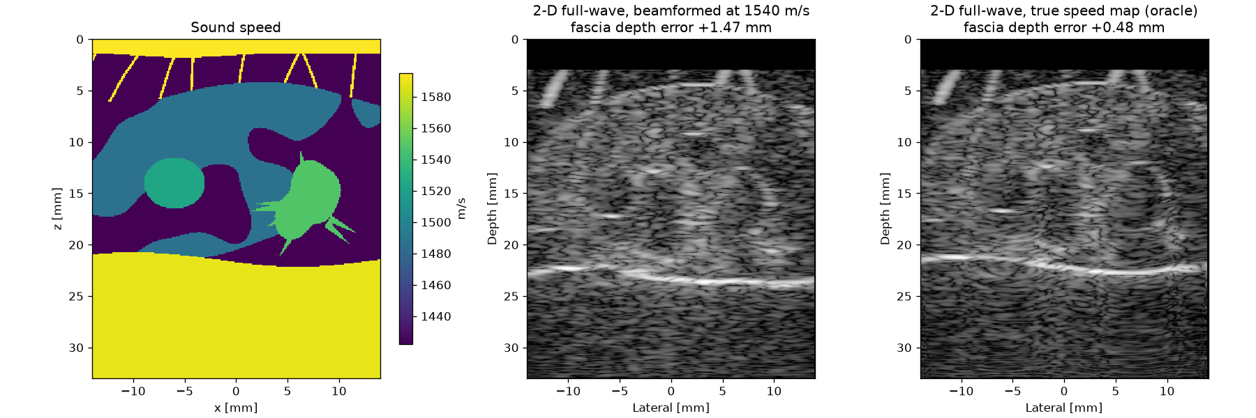
In 2-D every inclusion is an infinite cylinder: a cyst wall reflects and focuses coherently and fills the cyst with reverberation that a 3-D cyst would not have. The breast example below is therefore an aberration study: it measures how far the pectoralis fascia is displaced with 1540 m/s delays and with delays through the true speed map.

Nonlinear heating

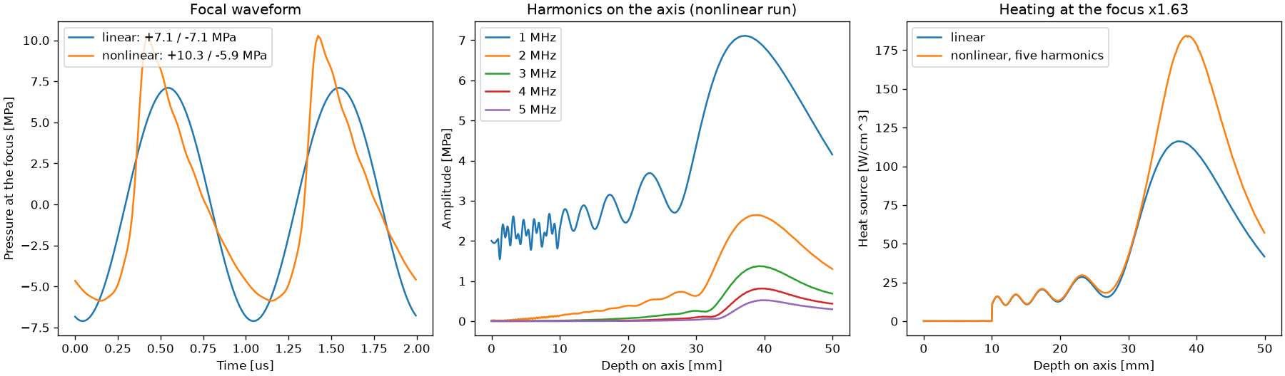
With nonlinear=True and cw=[f, 2f, 3f, ...], the harmonics of a focused beam come out as complex amplitude maps. thermal.heat_source_harmonics(res.cw, medium) adds their heating, each at its own attenuation.

Checks

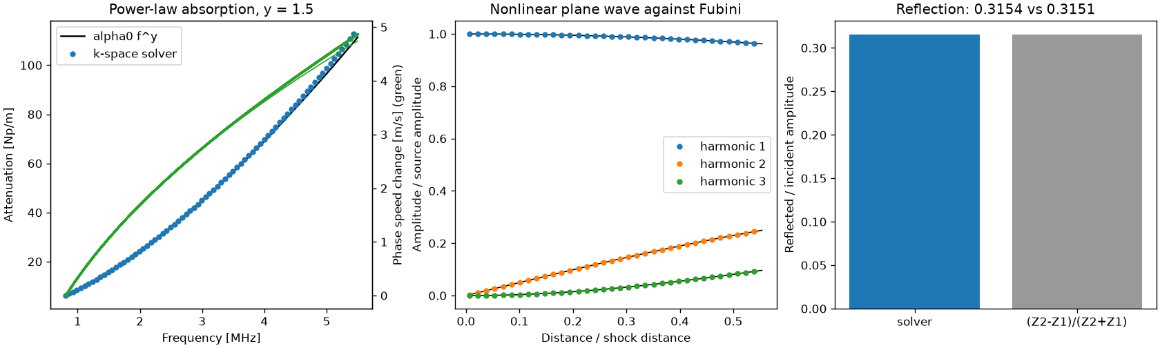
The Benchmarks page has the convergence study, the reflection of the absorbing layer and a comparison with k-Wave on a shared heterogeneous case. The tests compare arrival times and amplitudes in 1-D and 2-D, power-law attenuation (within 2.5 % from 1 to 5 MHz at four points per wavelength), the phase speed against the Kramers-Kronig relation (within 0.15 m/s), the reflection coefficient of an interface (0.5 %), the first three harmonics of a plane wave against the Fubini solution (within 0.002 of the source amplitude up to half the shock distance), single against double precision, and the position of a point target in a full-wave image.

Run time

Each time step costs about ten FFTs of the padded grid. A 2-D grid of 400 by 450 points takes about 15 ms per step in single precision with scipy installed, so a 4 MHz pulse-echo transmit through 35 mm of tissue takes about half a minute. 3-D grids are possible but large; the hybrid angular spectrum method in sonosk.field is the fast choice for 3-D therapy fields.

References

Tabei M., Mast T.D., Waag R.C. A k-space method for coupled first-order acoustic propagation equations. J. Acoust. Soc. Am. 111(1):53-63, 2002.

Treeby B.E., Cox B.T. Modeling power law absorption and dispersion for acoustic propagation using the fractional Laplacian. J. Acoust. Soc. Am. 127(5):2741-2748, 2010.

Treeby B.E., Jaros J., Rendell A.P., Cox B.T. Modeling nonlinear ultrasound propagation in heterogeneous media with power law absorption using a k-space pseudospectral method. J. Acoust. Soc. Am. 131(6):4324-4336, 2012.